 Software Required for Download – QGIS & R
※Applicable Version: QGIS Greater Than 3.16 & R Greater Than 3.0.0
Ⅰ. Introduction
GTWR
GTWR (Geographically and Temporally Weighted Regression) is an extension of GWR, standing for Geographically Weighted Regression. It's a statistical method used in Geographic Information Science (GIS) to explore spatial data relationships.
GTWR not only considers the impact of geographical location on the response variables but also takes into account the temporal factor. It can handle variations in both space and time simultaneously, such as the spread of diseases, fluctuations in the real estate market, etc. These patterns may vary due to differences in time and space.
Main Features and Considerations:
1.Spatial and Temporal Weights: It uses geographical and temporal weights to calculate regression parameters for each location and time point. This means that relatively closer observations (either in space or time) have a greater influence on the regression parameters of that point.
2.Model Interpretation: GTWR, similar to GWR, can produce parameter maps, showing how a specific parameter changes with geographical location and time, aiding in explaining spatial variability.
3.Data Requirements: Given the complexity of the GTWR model, it requires a large amount of data to ensure the stability and reliability of the results. Also, the data should cover a sufficient time span and spatial scope to accurately estimate model parameters.
4.High Computational Load: GTWR requires more computational resources as it has a regression equation for each geographical location and time point.
Plugin Advantage
1.User-Friendly
Users only need to install R and QGIS. After installing the Processing R Provider plugin in QGIS, just copy the relevant script files to the designated directory and you're set. If any changes or adjustments are needed later, you can directly modify the script files.
2.Time Clustering
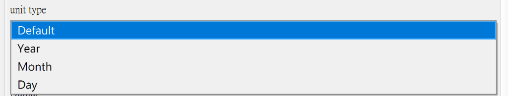
Users can group the temporal variables in the data based on their needs, whether it's daily, monthly, yearly, or by periods. For instance, you can group every five days as a new time variable, or consolidate daily data into monthly data. Users can adjust the desired unit (year, month, day, or the default data unit) and intervals. Once selected, the GTWR model will use the newly established time grouping as the time variable.
※ If the original data's time variable is on a larger scale, such as years or months, you can't select a smaller unit like months or days. If the data is in non-date formats like periods, you're limited to choosing the default data unit.
3.Model Visualization
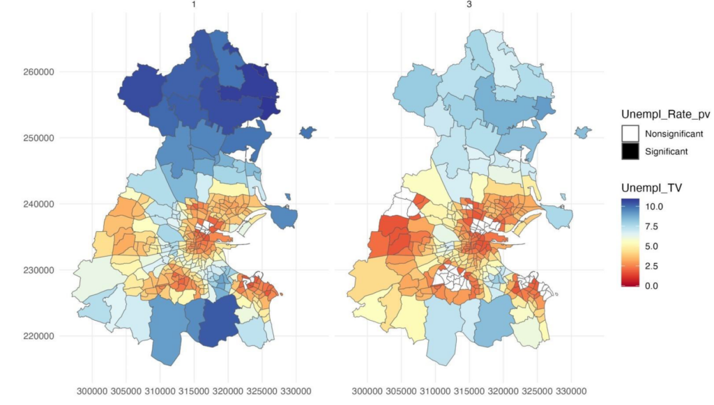
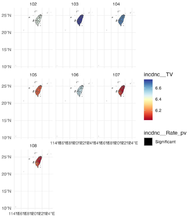
After executing the procedure, visualization images of the T-value results for each explanatory variable across various locations and times will be added to the folder specified by the user. If a location is significant for a particular explanatory variable, it will be colored based on the magnitude of the T-value. If it's not significant, the location will be colored white.
4.QGIS Variable Name Truncation Issue
When processing data, QGIS truncates variable names that exceed ten characters. However, in the parameter menu, the original full variable names are retained. Therefore, this procedure also truncates the variable names selected by the user in the manner of QGIS to prevent issues arising from discrepancies between the backend data variables in QGIS and the user's selection. Nevertheless, since QGIS's truncation method is related to the order of the variables, problems may still arise if the user's selected variable order differs from the original data's variable order.
Ⅱ. 安裝流程 (For Mac User)
Step 1
Install QGIS & R
Step 2
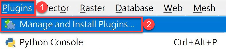
After opening QGIS, click on 'Plugins' in the top menu, then select 'Manage and install Plugins'.
Step 3
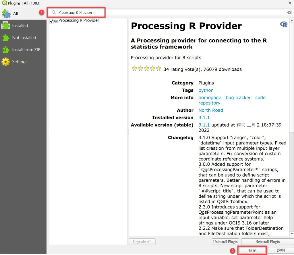
Search for 'Processing R Provider', then click on 'Install Plugin' > 'Close'.
Step 4
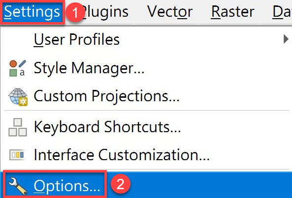
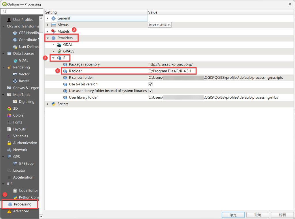
After restarting QGIS, click on 'Setting' > 'Options' in the top menu.
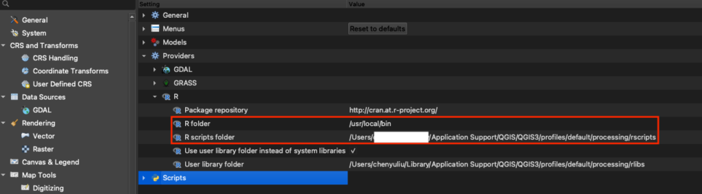
Step 5
Click on 'Processing' > 'Providers' > 'R', and set the R folder path (e.g., C:\Program Files\R\R-4.3.1; the actual path may vary depending on the system, version, or directory).
※If the installed R version is 64 bit, make sure to check the 'Use 64 bit version' option.
Step 6
Open the folder named 'R scripts folder'.
※This folder is used to store GWR or other R program files (the path is under the QGIS installation directory).
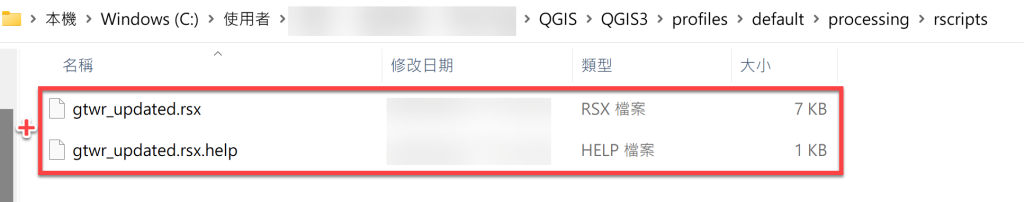
Step 7
Add gtwr.rsx and gtwr.help program files under the R scripts folder directory.
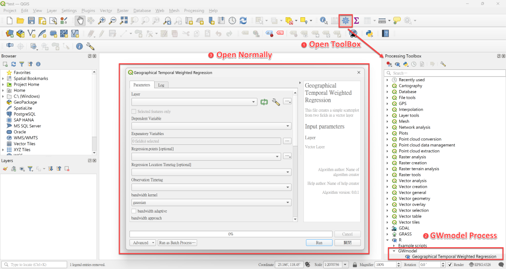
Step 8
Restart QGIS and verify in the Processing ToolBox whether the R category and the GWmodel folder within it have been successfully installed. If you see the Geographically and Temporally Weighted Regression program within the GWmodel category and it can be opened normally, it indicates the installation is complete.
※ If there's an issue when starting the Geographical and Temporal Weighted Regression program, the problem might be with the R folder path from Step 2.
Ⅲ. Example Operation
Step 1 Input Data
● Import spatiotemporal point data or spatiotemporal polygon data.
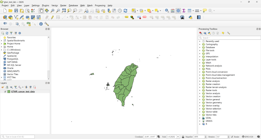
● After importing the data, launch the Geographical Temporal Weighted Regression process and select the input data in the Layer section.

Step 2 Select Parameters
This section is the primary user interface. Users can select the corresponding parameters and inputs based on their needs, and define the output data path.
● Dependent Variable
All variables are single-choice menus, allowing you to select the corresponding response variable according to your needs.

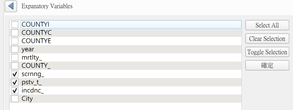
● Expanatory Variables
All variables are multiple-choice menus, allowing you to select the corresponding explanatory variables according to your needs.
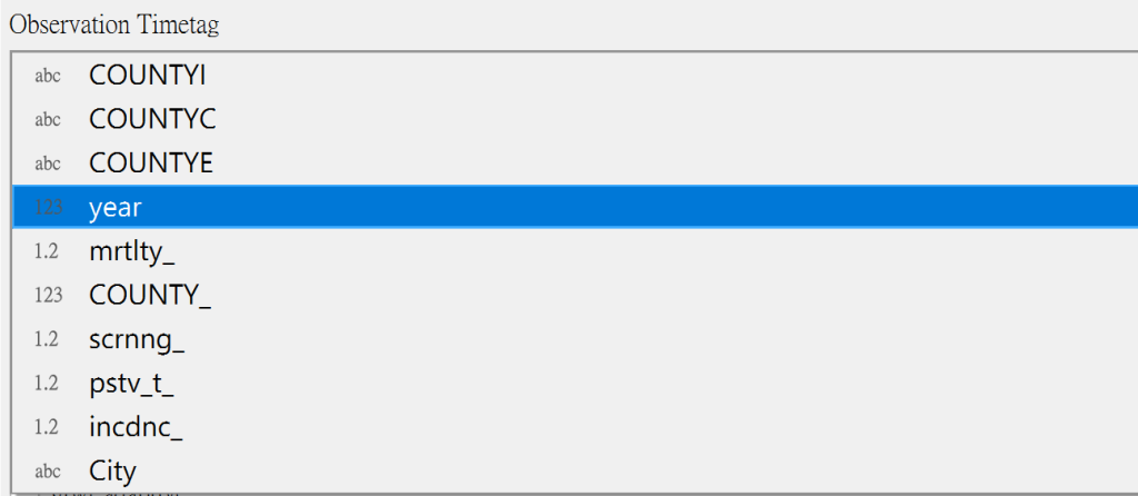
● Observation Timetag
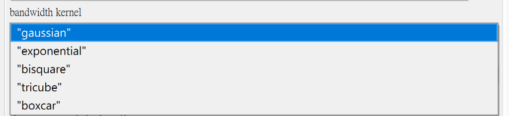
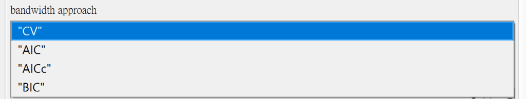
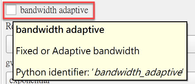
● Selection of Kernel, Approach, and Fixed / Adaptive
Select the parameters for calculating Bandwidth and the subsequent model parameters.
○ List of Kernel Functions – Gaussian, Exponential, Bisquare, Tricube, and Boxcar.
○ GTWR Approach – CV, AIC, AICc, and BIC.
○ Fixed or Adaptive bandwidth
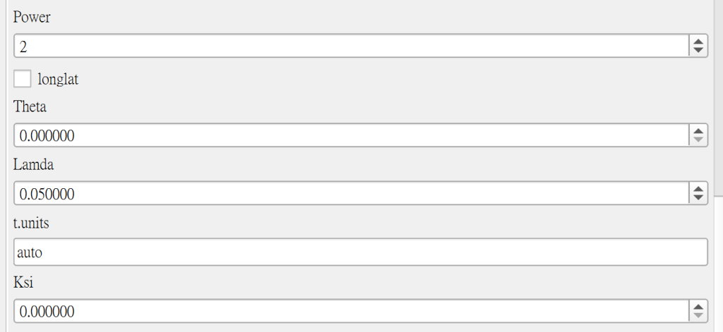
● Selection of Other Parameters
All have default values and can be adjusted according to the situation.
● Output Data Path
Specify the data output path.

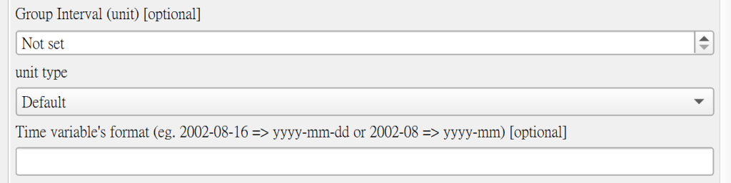
Step 3 Time Clustering
● You can choose whether to group the current time variable, for example, into new groups every five days or to aggregate monthly data into yearly or daily data into monthly data, and so on. Regardless of the data type, whether it's dates or periods, you can group them according to your needs. After grouping, the model will use the new grouped time variable for modeling.
● Users first need to choose the interval size and unit. It's important to note that the unit can only be chosen if it's larger than the scale of the time variable. For instance, if the time variable is daily, any unit can be selected. However, if the time variable is monthly, you can't choose a smaller scale like daily, and so on. If the time variable isn't in a date format, like periods, then select the "Default" unit. If the time variable is a date, you'll need to specifically input the date format.

Step 4 Output Results
● Document Output
During the process of running the procedure in QGIS, two main sets of data will be output:
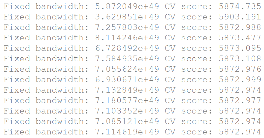
1. Scores for Different Bandwidths: Because of selecting a fixed bandwidth in the parameters and using CV scores for selection, the output results will contain various bandwidths and their corresponding scores (see lower left figure).
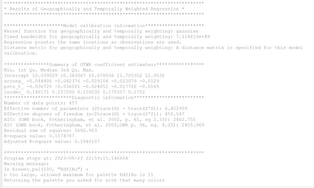
2. Model Results: The model provides basic information, such as AIC, AICc, R Squared, etc., as well as the maximum and minimum values of each coefficient (see the bottom right image). This content will also be exported as a document to the output path set by the user.
● Data Output
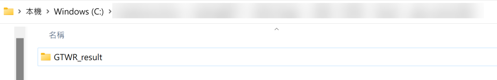
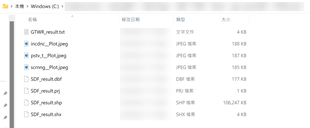
Upon completion of the process, a folder named 'GTWR_result' will be created in the user-specified path (see the bottom-left image). This folder contains three main sections of content:
1. "GWR_result.txt": Information document of the model (refer to the lower right figure).
2. Model output is in Shapefile format: It includes four files - 'SDF_reuslt.shp', 'SDF_result.shx', 'SDF_result.dbf', and 'SDF_result.prj'. If users want to utilize these files, they can import the 'SDF_result.shp' file into QGIS (see lower right figure). After the process is completed, QGIS will add a new 'Output' layer, with content identical to that of the 'SDF_result.shp' file, both representing the model's output result.
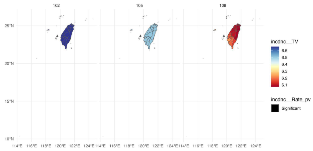
3. Visualization of the T-values for each explanatory variable in the model at various time points: If the test result for a specific region or point is not significant, no color will be displayed. Conversely, if it is significant, different colors and shades will be shown based on the magnitude of the value. If users have segmented the time, the visualization results at different time points will vary. The bottom left image shows the visualization results without time segmentation, while the bottom right image displays results grouped in three-year intervals.
For more information, you can refer the following:
[1] Chan, T. C., Chiang, P. H., Su, M. D., Wang, H. W., & Liu, M. S. Y. (2014). Geographic disparity in chronic obstructive pulmonary disease (COPD) mortality rates among the Taiwan population. PloS one, 9(5), e98170.
[2] Fotheringham, A. S., Crespo, R., & Yao, J. (2015). Geographical and temporal weighted regression (GTWR). Geographical Analysis, 47(4), 431-452.
[3] Nugroho, W. H., & Sumarminingsih, E. (2021, March). Geographically and Temporally Weighted Regression Model with Gaussian Kernel Weighted Function and Bisquare Kernel Weighted Function. In IOP Conference Series: Materials Science and Engineering (Vol. 1115, No. 1, p. 012063). IOP Publishing.
[4] Wu, B., Li, R., & Huang, B. (2014). A geographically and temporally weighted autoregressive model with application to housing prices. International Journal of Geographical Information Science, 28(5), 1186-1204.